7. The analyse command

snptoolkit analyse -h
usage: snptoolkit analyse [-h] -p POLYMORPHIC_SITES [-c CONFIG]

optional arguments:
-h, --help            show this help message and exit

snpToolkit analyze required options:
-p POLYMORPHIC_SITES  provide the path of the polymorphic sites you want to analyze
-c CONFIG             provide the path of the configuration file that contains the information to use for data visualization

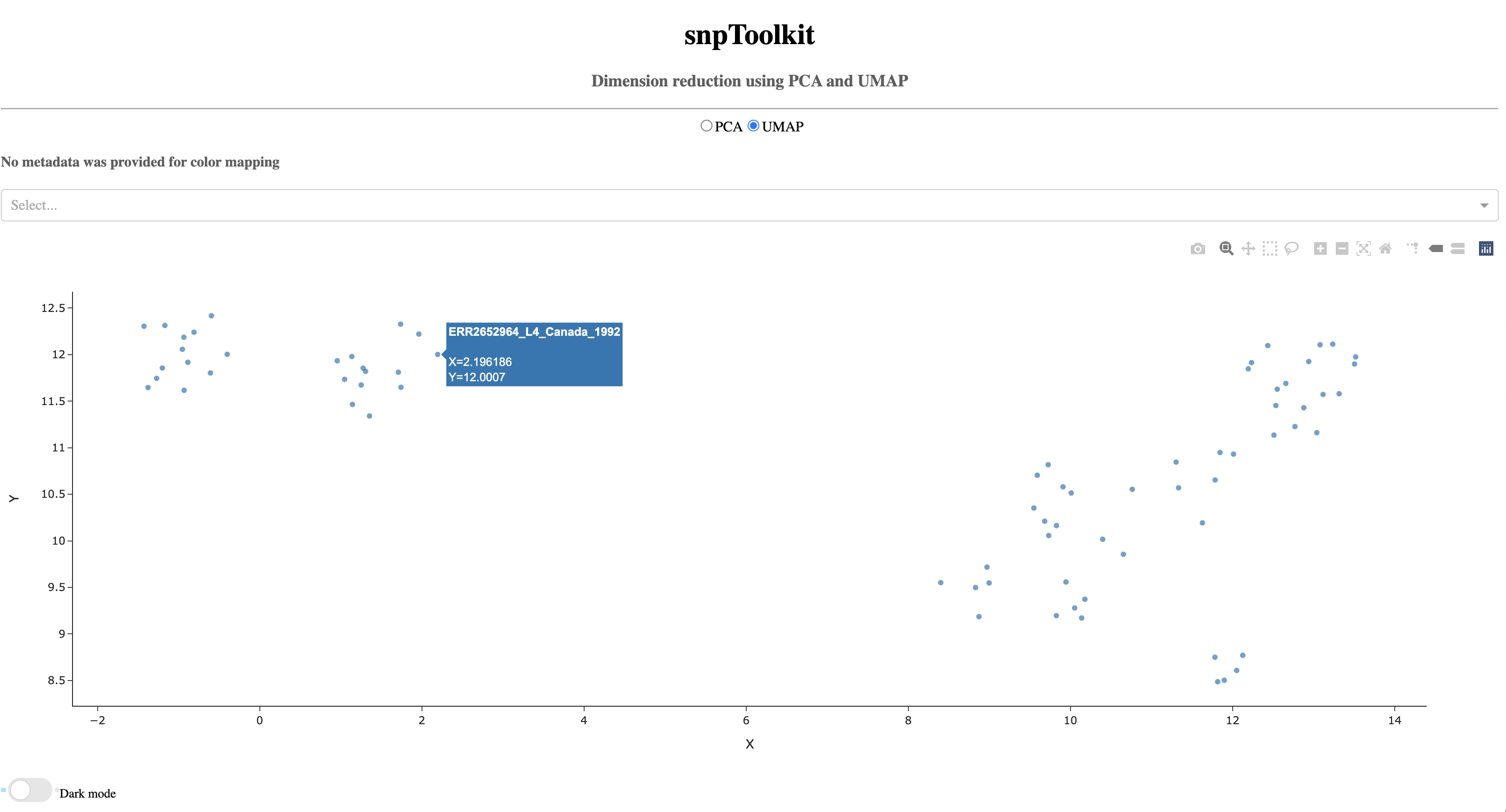
The main goal of this analysis is to use two dimentionality reduction methods: PCA and UMAP to cluster all your samples based on the distibution of all identified polymorphic sites between them. Principal Component analysis (PCA) is a quite knowing method and is an unsupervised linear dimensionality reduction and data visualization technique. On the other hand, UMAP is a Uniform Manifold Approximation and Projection for Dimension Reduction. From a visualization point of view, PCA tries to preserve the global structure of the data while UMAP tries to preserve global and local structure. To apply both of these methods you need to provide as input the file SNPs_polymorphic_sites.txt generated with the snptoolkit combine command.

$ snptoolkit analyse -p SNPs_polymorphic_sites.txt
Dash is running on http://127.0.0.1:8050/

* Serving Flask app "plot_polySites_output" (lazy loading)
* Environment: production
   WARNING: This is a development server. Do not use it in a production deployment.
   Use a production WSGI server instead.
* Debug mode: off
* Running on http://127.0.0.1:8050/ (Press CTRL+C to quit)

Note

In case you used the option –bam with the snptoolkit combine command, two output files will be generated: SNPs_polymorphic_sites.txt and SNPs_polymorphic_sites_clean.txt. The file SNPs_polymorphic_sites_clean.txt does not contains any missing information indicated with a question mark “?” and should be used as input file for dimentionality reduction.

After running the command snptoolkit analyse -p SNPs_polymorphic_sites.txt, you can access your result following the link http://127.0.0.1:8050/.

Note

Please note that this step may take some time depending on the size of your data.

The result will be displayed as follows:

7.1. PCA

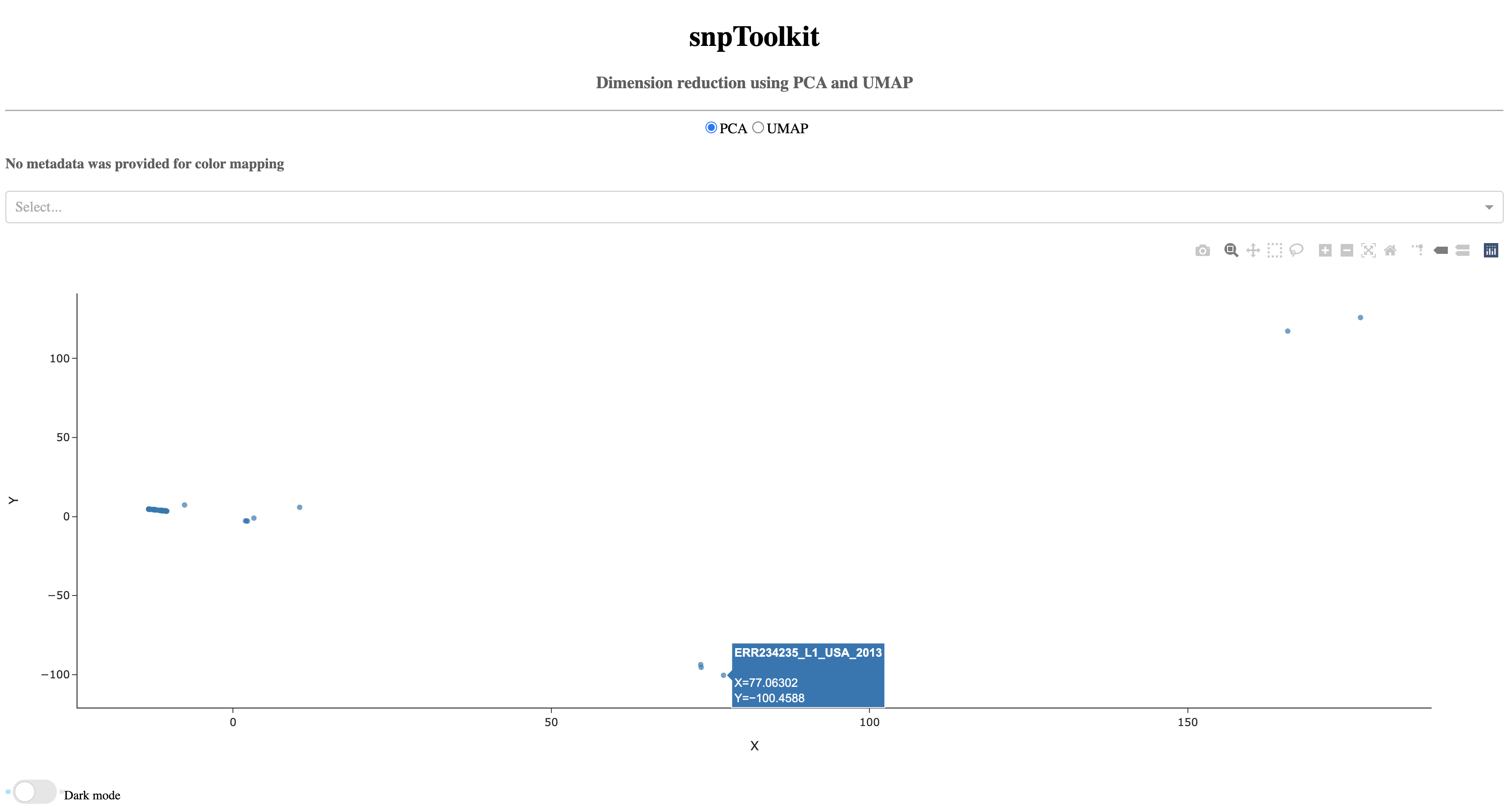
As you notice, when you hover of each dot, the name of the corresponding sample will be displayed.

7.2. UMAP

7.3. Color mapping

To take a better advantage of these two methods, it is possible to provide a configuration file that contains the metadata about the analyzed samples. This information will be used for color mapping which will make the visualization more comprehensive. The configuration file is a tab delimited file. Here is an example:

$ less metadata_file
         Lineage Rifampicin      Isoniazid       Pyrazinamide    Ethambutol      compensatory    Location        MDR
ERR760737_L4_Argentina_2006     L4      R       R       S       R       YES     Argentina       RR
ERR037537_L4_Malawi_0   L4      S       S       S       S       NO      Malawi  SS
ERR2652979_L4_Brazil_2004       L4      S       S       S       S       NO      Brazil  SS
ERR2652959_L4_Canada_2003       L4      S       S       S       S       NO      Canada  SS
ERR2653008_L4_Brazil_2004       L4      S       S       S       S       YES     Brazil  SS
ERR2652915_L4_USA_1999  L4      S       S       S       S       NO      USA     SS
ERR245833_L1_Malawi_0   L1      S       S       S       S       YES     Malawi  SS
ERR037471_L4_Malawi_0   L4      S       S       S       S       NO      Malawi  SS
ERR037549_L4_Malawi_0   L4      S       S       S       S       YES     Malawi  SS
ERR245675_L1_Malawi_0   L1      S       S       S       S       YES     Malawi  SS
ERR760755_L4_Argentina_2006     L4      R       R       S       R       YES     Argentina       RR

Note

Please note that the configuration file must contains all the samples that are present in the input file SNPs_polymorphic_sites.txt. In case not all the information is availble, you can just any label on the corresponding cells e.g. NA for not availble.

lets run the command analyse with the configuration file:

$ snptoolkit analyse -p SNPs_polymorphic_sites.txt -c metadata_file

Dash is running on http://127.0.0.1:8050/

* Serving Flask app "plot_polySites_output" (lazy loading)
* Environment: production
   WARNING: This is a development server. Do not use it in a production deployment.
   Use a production WSGI server instead.
* Debug mode: off
* Running on http://127.0.0.1:8050/ (Press CTRL+C to quit)

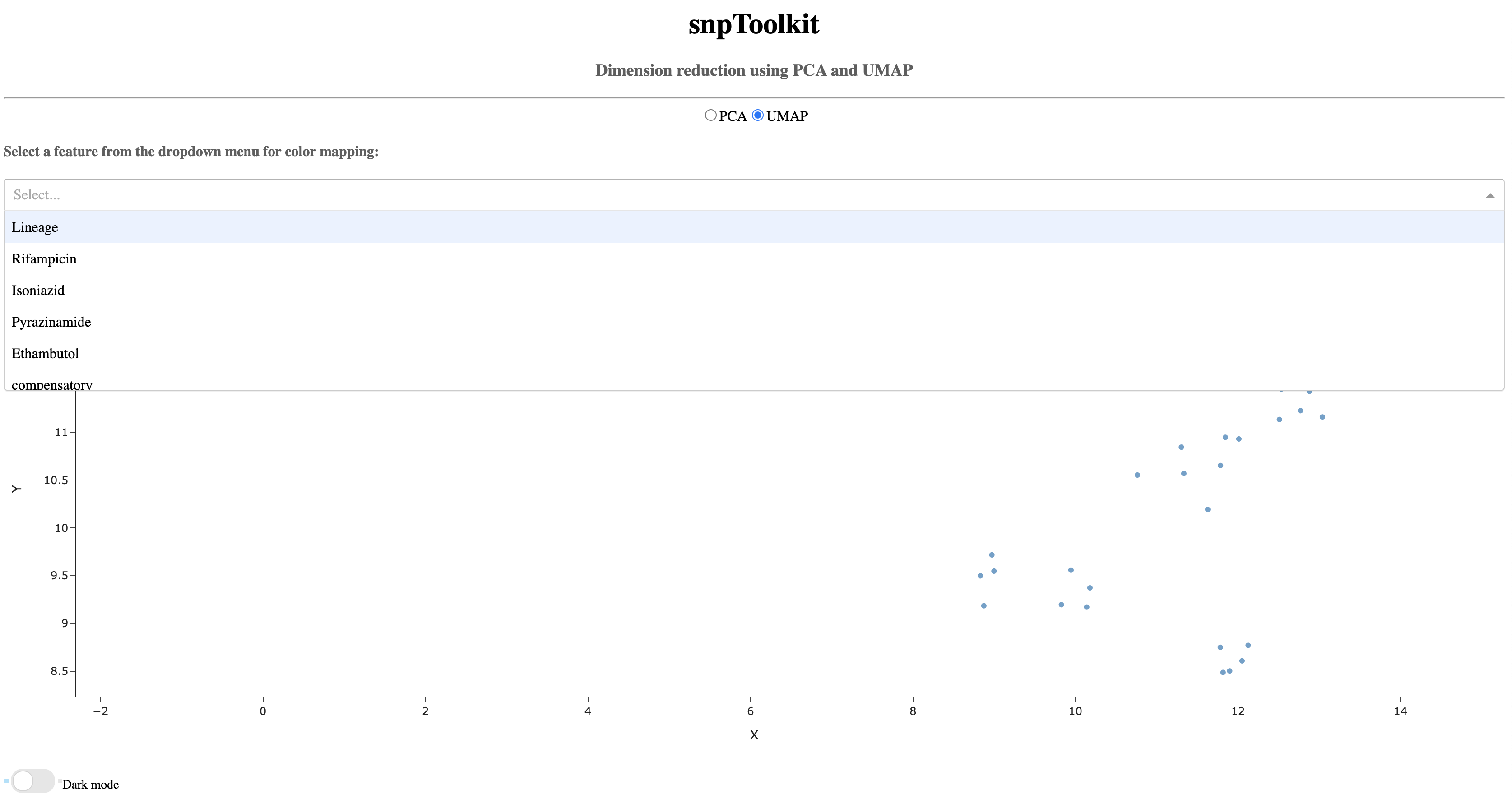
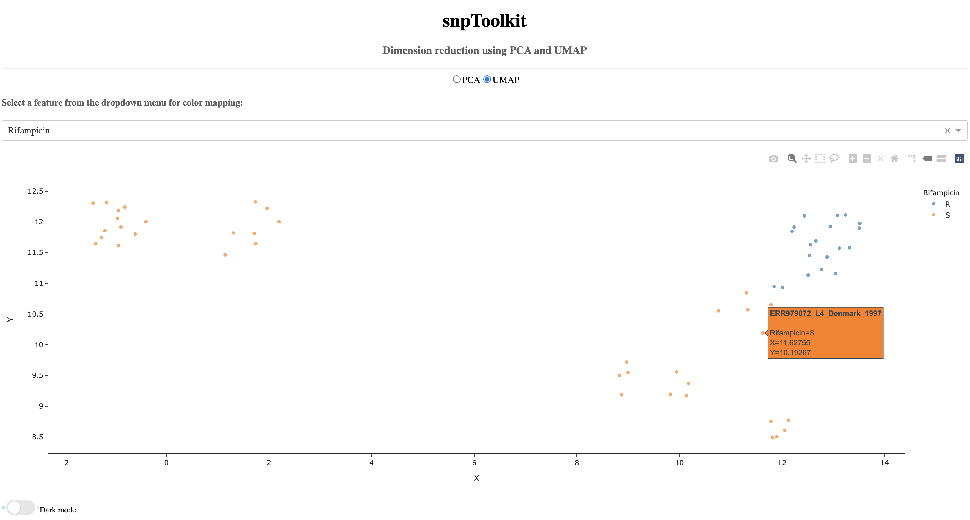
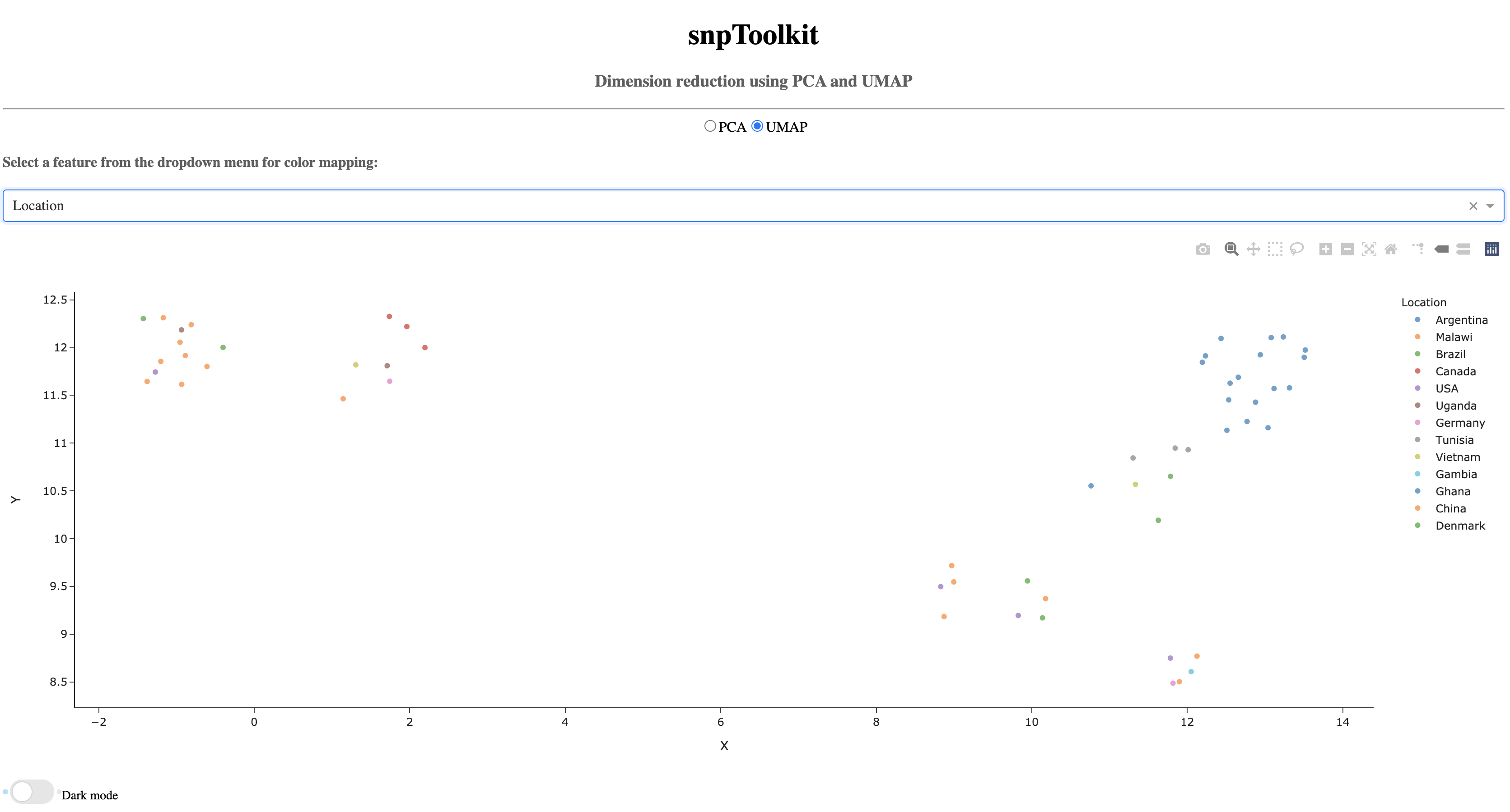
As you can see below, now the dropdown menu shows the list of features to use for coloring the different samples.

Now lets color the samples based on their resistance to rifampicin

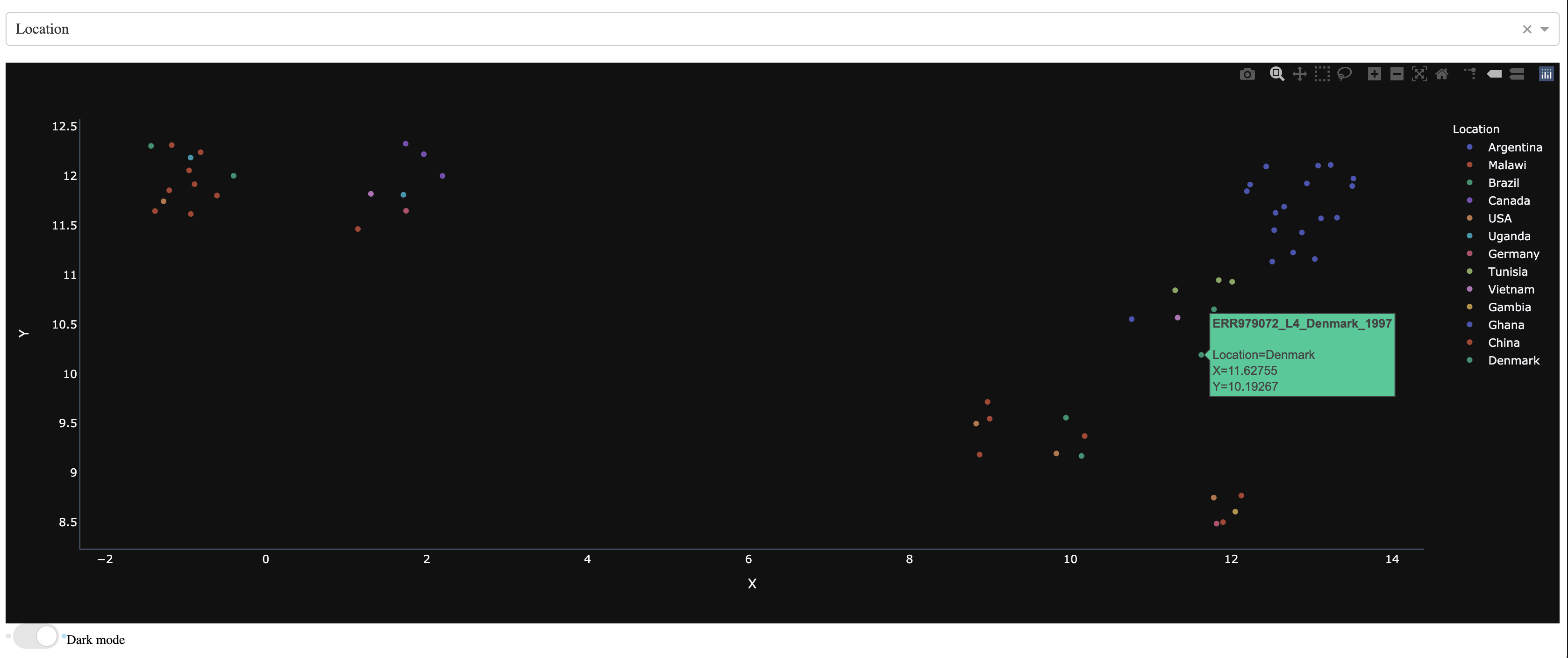
Now lets color the samples based on their location

For those (like me) that like dark mode in general you can turn it on to get graphs with dark bakground.